Electric Flux Through A Cube

half dozen.2: Electric Flux

Last updated
Salvage as PDF

Folio ID: 4379

Learning Objectives

Past the end of this section, you will exist able to:

Define the concept of flux
Describe electric flux
Calculate electric flux for a given state of affairs

The concept of flux describes how much of something goes through a given area. More than formally, it is the dot product of a vector field (in this affiliate, the electric field) with an surface area. You lot may conceptualize the flux of an electrical field as a measure of the number of electric field lines passing through an expanse (Figure \(\PageIndex{ane}\)). The larger the area, the more field lines get through it and, hence, the greater the flux; similarly, the stronger the electric field is (represented by a greater density of lines), the greater the flux. On the other hand, if the area rotated so that the plane is aligned with the field lines, none will pass through and at that place volition be no flux.

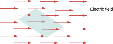
Figure shows a shaded area in the center. Several arrows pointing right are shown behind, in front of and passing through the shaded area. These are labeled electric field. — Figure \(\PageIndex{1}\): The flux of an electrical field through the shaded surface area captures information about the "number" of electrical field lines passing through the area. The numerical value of the electric flux depends on the magnitudes of the electrical field and the surface area, too every bit the relative orientation of the surface area with respect to the direction of the electric field.

A macroscopic analogy that might help you imagine this is to put a hula hoop in a flowing river. Equally you change the angle of the hoop relative to the direction of the current, more or less of the period will go through the hoop. Similarly, the amount of flow through the hoop depends on the strength of the current and the size of the hoop. Again, flux is a general concept; we can likewise use it to draw the amount of sunlight striking a solar panel or the amount of energy a telescope receives from a distant star, for example.

To quantify this thought, Figure \(\PageIndex{1a}\) shows a planar surface \(S_1\) of surface area \(A_1\) that is perpendicular to the uniform electric field \(\vec{E} = East\chapeau{y}\). If N field lines pass through \(S_1\), and then we know from the definition of electric field lines (Electric Charges and Fields) that \(North/A \propto East\), or \(N \propto EA_1\).

The quantity \(EA_1\) is the electric flux through \(S_1\). Nosotros correspond the electric flux through an open surface like \(S_1\) past the symbol \(\Phi\). Electric flux is a scalar quantity and has an SI unit of newton-meters squared per coulomb (\(N \cdot m^2/C\)). Observe that \(N \propto EA_1\) may also be written every bit \(N \propto \Phi\), demonstrating that electric flux is a measure out of the number of field lines crossing a surface.

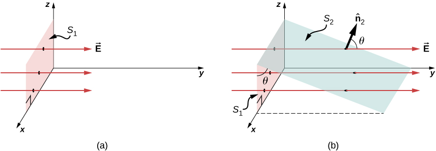
Figure a shows a rectangular shaded area in the xz plane. This is labeled S1. There are three arrows labeled E passing through S1. They are parallel to the y axis and point along the positive y axis. Figure b, too has plane S1 and arrows E. Another plane, labeled S2 forms an angle theta with plane S1. Their line of intersection is parallel to the x axis. An arrow labeled n hat 2 forms an angle theta with E. — Figure \(\PageIndex{two}\): (a) A planar surface \(S_1\) of surface area \(A_1\) is perpendicular to the electrical field \(Eastward\hat{j}\). N field lines cross surface \(S_1\). (b) A surface \(S_2\) of expanse \(A_2\) whose projection onto the xz-plane is \(S_1\). The same number of field lines cantankerous each surface.

At present consider a planar surface that is not perpendicular to the field. How would nosotros represent the electric flux? Figure \(\PageIndex{2b}\) shows a surface \(S_2\) of expanse \(A_2\) that is inclined at an angle \(\theta\) to the xz-plane and whose project in that plane is \(S_1\) (area \(A_1\)). The areas are related by \(A_2 \, cos \, \theta = A_1\). Considering the same number of field lines crosses both \(S_1\) and \(S_2\), the fluxes through both surfaces must be the same. The flux through \(S_2\) is therefore \(\Phi = EA_1 = EA_2 \, cos \, \theta\). Designating \(\hat{due north}_2\) as a unit vector normal to \(S_2\) (encounter Effigy \(\PageIndex{2b}\)), nosotros obtain

\[\Phi = \vec{E} \cdot \lid{n}_2 A_2.\]

Note

Cheque out this video to discover what happens to the flux as the area changes in size and angle, or the electrical field changes in strength.

Area Vector

For discussing the flux of a vector field, information technology is helpful to introduce an area vector \(\vec{A}\). This allows us to write the final equation in a more compact course. What should the magnitude of the expanse vector be? What should the direction of the expanse vector be? What are the implications of how you answer the previous question?

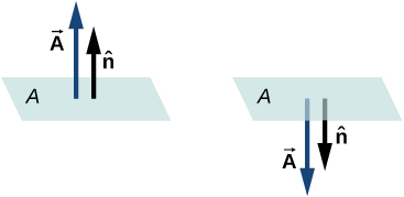
The area vector of a apartment surface of area A has the post-obit magnitude and management:

Magnitude is equal to area (A)
Direction is along the normal to the surface \((\hat{n})\); that is, perpendicular to the surface.

Since the normal to a flat surface can point in either management from the surface, the direction of the surface area vector of an open surface needs to be chosen, equally shown in Figure \(\PageIndex{3}\).

Figure shows two horizontal planes labeled A. The first has two arrows pointing up from the plane. The longer is labeled vector A and the shorter is labeled n hat. The second plane has the same two arrows pointing down from the plane. — Effigy \(\PageIndex{3}\): The direction of the area vector of an open surface needs to exist chosen; information technology could be either of the 2 cases displayed here. The area vector of a part of a closed surface is defined to point from the inside of the closed infinite to the outside. This rule gives a unique direction.

Since \(\lid{n}\) is a unit of measurement normal to a surface, it has two possible directions at every point on that surface (Figure \(\PageIndex{1a}\)). For an open surface, we can employ either direction, equally long as nosotros are consistent over the entire surface. \(\PageIndex{1c}\) of the figure shows several cases.

Figure a shows a curved rectangular surface. Two arrows originate from a point at its center and point in opposite directions. They are both perpendicular to the surface. They are labeled n hat 1 and n hat 2. Figure b shows a 3 dimensional surface shaped somewhat like a light bulb. There are five arrows labeled n hat, which originate from various points on the surface and point outward, perpendicular to the surface. Figure c shows three rectangular surfaces labeled S1, S2 and S3. Two arrows labeled n hat are perpendicular to S1 and point in opposite directions. Three arrows labeled n hat are perpendicular to S2, one pointing in a direction opposite to the other two. There are three arrows perpendicular to S3. All point outward from the same side of the surface. — Figure \(\PageIndex{four}\): (a) Two potential normal vectors arise at every point on a surface. (b) The outward normal is used to calculate the flux through a closed surface. (c) Simply \(S_3\) has been given a consistent fix of normal vectors that allows us to define the flux through the surface.

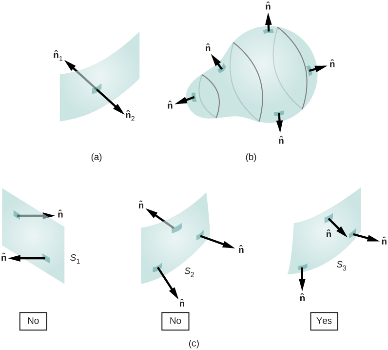
Still, if a surface is closed, and then the surface encloses a volume. In that case, the direction of the normal vector at any point on the surface points from the inside to the outside. On a closed surface such every bit that of Figure \(\PageIndex{1b}\), \(\chapeau{n}\) is called to be the outward normal at every point, to be consequent with the sign convention for electrical charge.

Electric Flux

Now that nosotros have defined the area vector of a surface, we can define the electric flux of a uniform electric field through a flat area as the scalar product of the electric field and the area vector:

\[\Phi = \vec{E} \cdot \vec{A} \, (compatible \, \chapeau{E}, \, flat \, surface).\]

Figure \(\PageIndex{5}\) shows the electric field of an oppositely charged, parallel-plate arrangement and an imaginary box between the plates. The electric field between the plates is uniform and points from the positive plate toward the negative plate. A adding of the flux of this field through diverse faces of the box shows that the net flux through the box is nix. Why does the flux cancel out here?

A cube ABCDKFGH is shown in the center. A diagonal plane is shown within it from KF to BC. The top surface of the cube, FGHK has a plane labeled minus q slightly above it and parallel to it. Similarly, another plane is labeled plus q is shown slightly below the bottom surface of the cube, parallel to it. Small red arrows are shown pointing upwards from the bottom plane, pointing up to the bottom surface of the cube, pointing up from the top surface of the cube and pointing up to the top plane. These are labeled vector E. — Figure \(\PageIndex{five}\): Electric flux through a cube, placed between two charged plates. Electric flux through the bottom face (**ABCD**) is negative, because \(\vec{Eastward}\) is in the reverse direction to the normal to the surface. The electric flux through the height face up (**FGHK**) is positive, considering the electric field and the normal are in the same management. The electric flux through the other faces is zero, since the electrical field is perpendicular to the normal vectors of those faces. The net electric flux through the cube is the sum of fluxes through the half dozen faces. Here, the internet flux through the cube is equal to zilch. The magnitude of the flux through rectangle **BCKF** is equal to the magnitudes of the flux through both the top and lesser faces.

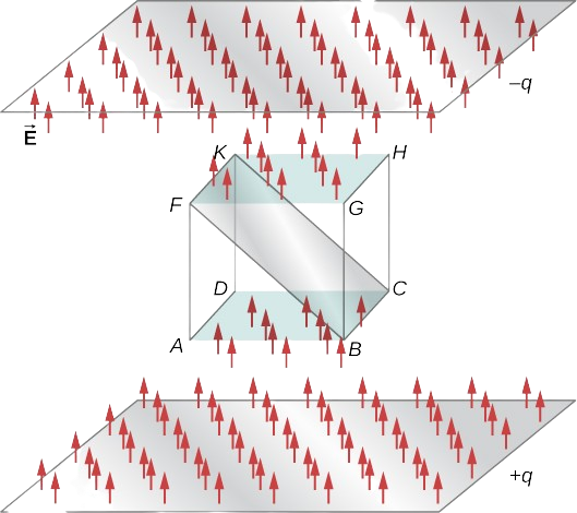
The reason is that the sources of the electrical field are outside the box. Therefore, if any electric field line enters the volume of the box, it must also go out somewhere on the surface because at that place is no accuse inside for the lines to land on. Therefore, quite more often than not, electrical flux through a closed surface is zilch if there are no sources of electrical field, whether positive or negative charges, inside the enclosed book. In full general, when field lines leave (or "flow out of") a closed surface, \(\Phi\) is positive; when they enter (or "menstruation into") the surface, \(\Phi\) is negative.

Any smooth, not-flat surface can exist replaced by a drove of tiny, approximately flat surfaces, as shown in Figure \(\PageIndex{6}\). If we split a surface S into pocket-sized patches, so we notice that, as the patches become smaller, they can be approximated past apartment surfaces. This is similar to the manner we treat the surface of Earth equally locally apartment, fifty-fifty though we know that globally, it is approximately spherical.

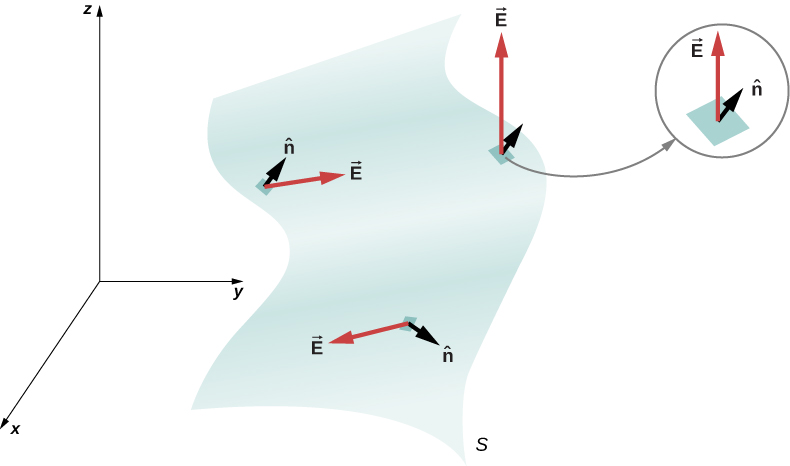
Figure shows a wavy surface labeled S. Three arrows labeled n hat originate from three different patches on the surface. Longer arrows labeled vector E also originate from each patch. An enlarged view of one patch is shown on the side. It shows n hat to be perpendicular to the patch. — Effigy \(\PageIndex{6}\): A surface is divided into patches to find the flux.

To keep track of the patches, we tin can number them from 1 through Due north . Now, we ascertain the area vector for each patch as the surface area of the patch pointed in the direction of the normal. Let united states denote the surface area vector for the ithursday patch past \(\delta \vec{A}_i\). (We have used the symbol \(\delta\) to remind u.s. that the expanse is of an arbitrarily small patch.) With sufficiently small patches, we may approximate the electric field over whatever given patch as compatible. Allow us denote the boilerplate electric field at the location of the ith patch past \(\vec{E}_i\).

\[\vec{Eastward}_i = \mathrm{average \, electric \, field \, over \, the \,} i \mathrm{thursday \, patch}.\]

Therefore, we tin write the electric flux \(\Phi\) through the area of the ith patch as

\[\Phi_i = \vec{E}_i \cdot \delta \vec{A}_i \, (i \mathrm{th \, patch}).\]

The flux through each of the individual patches tin exist constructed in this way and then added to requite us an estimate of the internet flux through the entire surface S, which nosotros announce just every bit \(\Phi\).

\[\Phi = \sum_{i=1}^Northward \Phi_i = \sum_{i=one}^N \vec{E}_i \cdot \delta \vec{A}_i \, (N \, patch \, guess).\]

This estimate of the flux gets better as we subtract the size of the patches. Nonetheless, when you use smaller patches, you lot need more than of them to cover the same surface. In the limit of infinitesimally small patches, they may be considered to accept area dA and unit of measurement normal \(\hat{n}\). Since the elements are infinitesimal, they may be causeless to exist planar, and \(\vec{E}_i\) may be taken as constant over whatever element. Then the flux \(d\Phi\) through an area dA is given by \(d\Phi = \vec{E} \cdot \hat{n} dA\). It is positive when the angle between \(\vec{E}_i\) and \(\hat{due north}\) is less than \(90^o\) and negative when the angle is greater than \(90^o\). The net flux is the sum of the infinitesimal flux elements over the entire surface. With infinitesimally small patches, you need infinitely many patches, and the limit of the sum becomes a surface integral. With \(\int_S\) representing the integral over S,

\[\Phi = \int_S \vec{E} \cdot \chapeau{due north}dA = \int_S \vec{Due east} \cdot d\vec{A} \, (open \, surface).\]

In practical terms, surface integrals are computed past taking the antiderivatives of both dimensions defining the area, with the edges of the surface in question being the bounds of the integral.

To distinguish between the flux through an open surface like that of Figure \(\PageIndex{2}\) and the flux through a closed surface (one that completely bounds some volume), nosotros represent flux through a closed surface by

\[\Phi = \oint_S \vec{E} \cdot \hat{n} dA = \oint_S \vec{E} \cdot d\vec{A} \, (closed \, surface)\]

where the circle through the integral symbol merely means that the surface is closed, and we are integrating over the entire thing. If you lot only integrate over a portion of a closed surface, that ways y'all are treating a subset of it every bit an open surface.

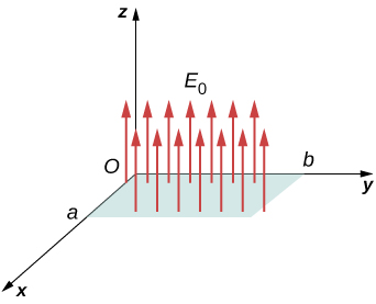
Example \(\PageIndex{one}\): Flux of a Uniform Electrical Field

A constant electric field of magnitude \(E_0\) points in the direction of the positive z-axis (Figure \(\PageIndex{7}\)). What is the electrical flux through a rectangle with sides a and b in the (a) xy-airplane and in the (b) xz-plane?

A rectangular patch is shown in the xy plane. Its side along the x axis is of length a and its side along the y axis is of length b. Arrows labeled E subscript 0 originate from the plane and point in the positive z direction. — Figure \(\PageIndex{7}\): Calculating the flux of \(E_0\) through a rectangular surface.

Strategy

Utilise the definition of flux: \(\Phi = \vec{E} \cdot \vec{A} \, (compatible \, \vec{Due east})\), where the definition of dot production is crucial.

Solution

In this case, \(\Phi = \vec{E}_0 \cdot \vec{A} = E_0 A = E_0 ab\).
Hither, the direction of the area vector is either along the positive y-centrality or toward the negative y-axis. Therefore, the scalar product of the electric field with the area vector is zero, giving zero flux.

Significance

The relative directions of the electric field and area can crusade the flux through the area to be nix.

Flux of a Uniform Electrical Field through a Closed Surface

A abiding electric field of magnitude \(E_0\) points in the direction of the positive z-centrality (Effigy \(\PageIndex{8}\)). What is the cyberspace electric flux through a cube?

Strategy

Utilise the definition of flux: \(\Phi = \vec{East} \cdot \vec{A} \, (uniform \, \vec{Due east})\), noting that a closed surface eliminates the ambiguity in the management of the area vector.

Solution

Through the acme face of the cube \(\Phi = \vec{E}_0 \cdot \vec{A} = E_0 A\).

Through the bottom confront of the cube, \(\Phi = \vec{E}_0 \cdot \vec{A} = - E_0 A\), because the area vector hither points downward.

Along the other four sides, the direction of the surface area vector is perpendicular to the direction of the electrical field. Therefore, the scalar product of the electric field with the area vector is zero, giving nix flux.

The internet flux is \(\Phi_{net} = E_0A - E_0 A + 0 + 0 + 0 + 0 = 0\).

Significance

The internet flux of a uniform electric field through a closed surface is zero.

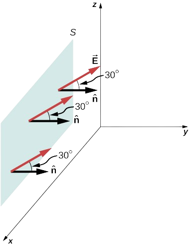
Example \(\PageIndex{three}\): Electric Flux through a Plane, Integral Method

A uniform electric field \(\vec{E}\) of magnitude 10 Northward/C is directed parallel to the yz-plane at \(30^o\) to a higher place the xy-airplane, as shown in Figure \(\PageIndex{9}\). What is the electric flux through the airplane surface of area \(half-dozen.0 \, m^2\) located in the xz-airplane? Assume that \(\hat{n}\) points in the positive y-direction.

A rectangular surface S is shown in the xz plane. Three arrows labeled n hat originate from three points on the surface and point in the positive y direction. Three longer arrows labeled vector E also originate from the same points. They make an angle of 30 degrees with n hat. — Figure \(\PageIndex{9}\): The electric field produces a cyberspace electric flux through the surface S.

Strategy

Utilise \(\Phi = \int_S \vec{E} \cdot \hat{n} dA\), where the direction and magnitude of the electric field are constant.

Solution

The angle betwixt the compatible electric field \(\vec{Eastward}\) and the unit normal \(\lid{n}\) to the planar surface is \(30^o\). Since both the direction and magnitude are abiding, E comes outside the integral. All that is left is a surface integral over dA, which is A. Therefore, using the open-surface equation, nosotros notice that the electric flux through the surface is

\[\Phi = \int_S \vec{E} \cdot \hat{north} dA = EA \, cos \, \theta\]

\[= (x \, North/C)(6.0 \, yard^2)(cos \, 30^o) = 52 \, North \cdot m^ii/C.\]

Significance

Again, the relative directions of the field and the area matter, and the general equation with the integral will simplify to the uncomplicated dot product of area and electric field.

Exercise \(\PageIndex{1}\)

What angle should there be between the electric field and the surface shown in Figure \(\PageIndex{9}\) in the previous case so that no electric flux passes through the surface?

Solution

Place it so that its unit normal is perpendicular to \(\vec{E}\).

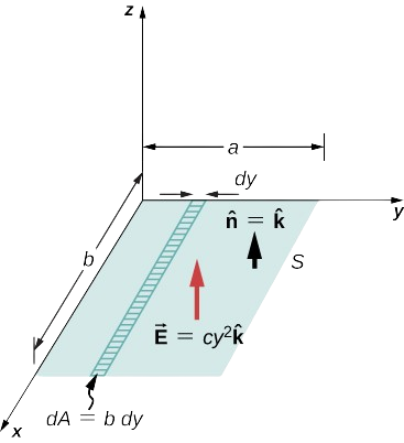
Example \(\PageIndex{4}\) : Inhomogeneous Electric Field

What is the total flux of the electric field \(\vec{Eastward} = cy^2\hat{1000}\) through the rectangular surface shown in Effigy \(\PageIndex{10}\)?

A rectangle labeled S is shown in the xy plane. Its side along y axis is of length a and that along the x axis measures b. A strip is marked on the rectangle, with its length parallel to x axis. Its length is b and its breadth is dy. Its area is labeled dA equal to b dy. Two arrows are shown perpendicular to S, n hat equal to k hat and vector E equal to cy squared k hat. These point in the positive z direction. — Figure \(\PageIndex{10}\): Since the electric field is non constant over the surface, an integration is necessary to determine the flux.

Strategy

Apply \(\Phi = \int_S \vec{Eastward} \cdot \hat{n}dA\). We assume that the unit normal \(\hat{n}\) to the given surface points in the positive z-management, so \(\hat{n} = \hat{k}\). Since the electric field is non compatible over the surface, it is necessary to split the surface into infinitesimal strips along which \(\vec{E}\) is essentially abiding. Equally shown in Figure \(\PageIndex{ten}\), these strips are parallel to the ten-axis, and each strip has an area \(dA = b \, dy\).

Solution

From the open surface integral, we find that the net flux through the rectangular surface is

\[\begin{marshal*} \Phi &= \int_S \vec{East} \cdot \hat{n} dA = \int_0^a (cy^2 \chapeau{one thousand}) \cdot \hat{k}(b \, dy) \\[4pt] &= cb \int_0^a y^2 dy = \frac{ane}{three} a^3 bc. \end{align*}\]

Significance

For a non-constant electric field, the integral method is required.

Exercise \(\PageIndex{one}\)

If the electrical field in Instance \(\PageIndex{4}\) is \(\vec{E} = mx\lid{k}\). what is the flux through the rectangular area?

Solution

\(mab^2/ii\)